
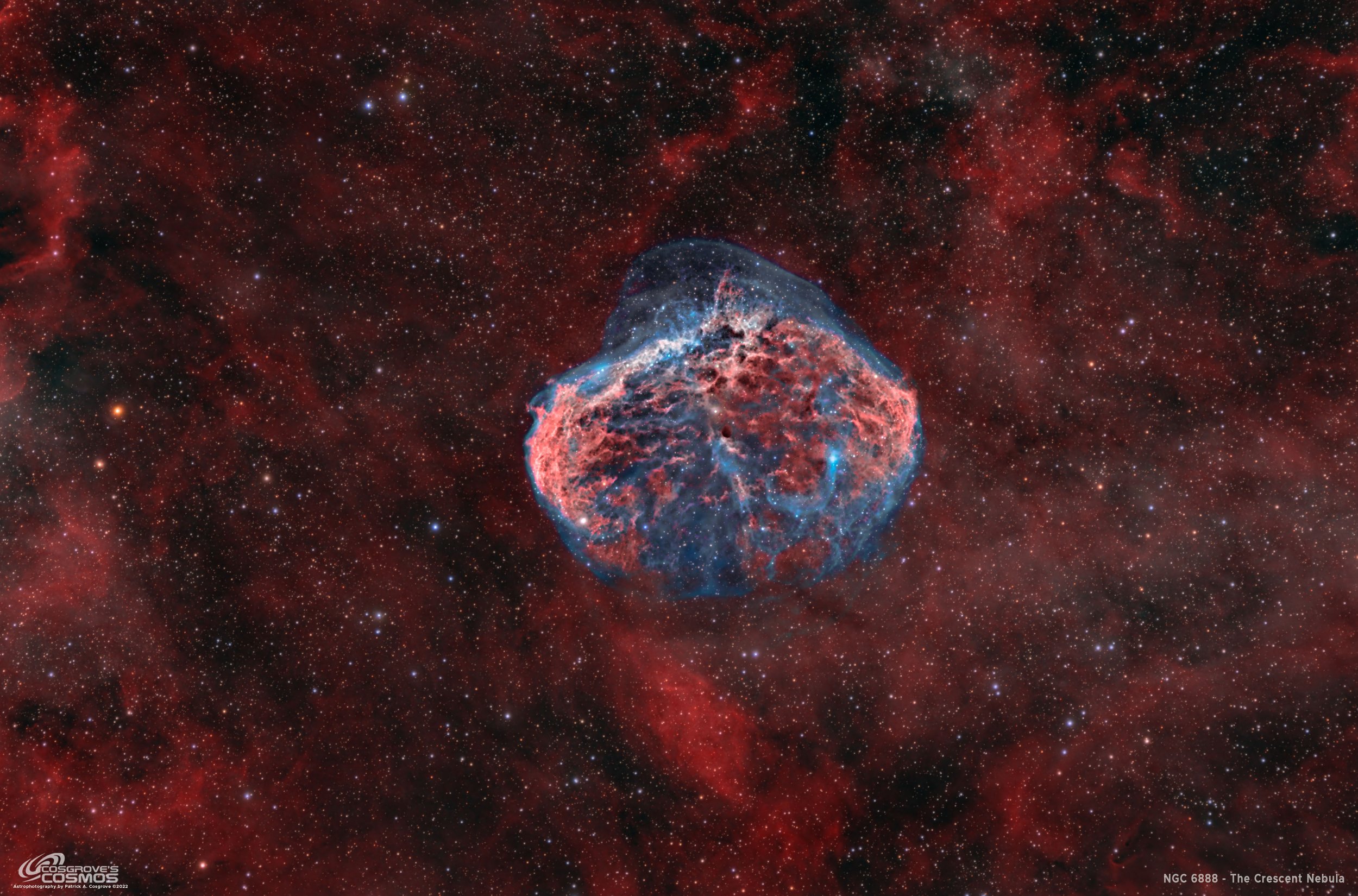
NGC 6888 - The Crescent Nebula - 12.9 hours in HOOrgb
Date: Sept 16, 2022
Cosgrove’s Cosmos Catalog ➤#0112

NGC 6888 - the Crescent Nebula in Bi-color - HOO - with RGB stars. The is a lot of Ha signal in this region, as you can see in the background sky! (click on the image for a full res version via Astrobin.com)
Published in Amateur Astrophotography Magazine!
April 9th, 2023 - In issue #111, p70-75. This image was published as part of a profile article on me!


Table of Contents Show (Click on lines to navigate)
Special Note
There has been a more recent Reprocessing Project for this image data. This is listed as its own project and can be seen HERE.
About the Target
NGC 6888 - The Crescent Nebula - is an emission nebula located about 5000 light-years away in the constellation of Cygnus. It is also known as Caldwell 27 and Sharpless 105.
This object can be seen visually with a modest telescope, which appears as a crescent shape - thus its name. This view can be improved by using a UHC or O-III filter.

Friedrich Wilhelm Herschel (1738-1822). Image taken from Wikipedia.
This object was discovered and cataloged by William Herschel in 1792.
Wikipedia it thusly:
It is formed by the fast stellar wind from the Wolf-Rayet star WR 136 (HD 192163) colliding with and energizing the slower moving wind ejected by the star when it became a red giant around 250,000 to 400,000 years ago. The result of the collision is a shell and two shock waves, one moving outward and one moving inward. The inward-moving shock wave heats the stellar wind to X-ray-emitting temperatures.
The Annotated Image

This annotated image was created using the Pixinsight ImageSolve and ImageAnnotation scripts.
The Location in the Sky

This finger chart was created in Pixinsight using the FinderChart process.
About the Project
Intro Video
A few minutes of introduction for this project by yours truly! While the processing walkthrough at the end of this post is quite detailed, sometimes it is hard to determine why some steps are done in the sequence they are. I wanted to find a way to have a 50,000-foot view and get a sense of the forest versus the trees.
So I created a high-level one-page map of the processing flow. You will see this map further into the post.
But this got me thinking about the video overviews I have been trying to include for each project.
I thought perhaps I could show this chart and walk folks through the processing steps - from a high-level perspective - and offer a view of where the image evolves as it is processed.
So this video is an experiment doing that. I hope it gives a good feel for my processing strategy and how the image goes from Master Linear images to the final image I share with you all.
Let me know if you like this approach, or if you have any suggestions as to how I might evolve the approach - I am all ears!
Finally, I would also ask you consider subscribing to my fledging YouTube Channel and “ring the notification bell”. This supports the channel, helping to position it with YouTube’s algorithms.
Thank you!
Choosing the Target
The constellation Cygnus has been positioned well for me during the last capture cycle, and as a result, I have been picking from the plentiful targets it holds.
I was looking for something suitable for my Astro-Physics 130mm platform with the ZWO ASI2600MM-Pro camera. When I came across NGC 6888, I paused for a moment. This was one of the early targets I shot when I first began to use a mono camera. It was my first bi-color image as well.
Astrophotographers sometimes like to revisit targets they have already shot and see how much better they can do with them - given improved gear, procedures, image processing, and more experience.
I suppose it’s a measure of progress and validation for our efforts.
That’s what motivated me here. I wanted to try this one again, putting my best foot forward and seeing what would come back!
Data Capture
I captured subs over four nights: Aug 24, Aug 28, Sept 1, and Sept 2.
In general, these nights were clear and cool. The first night was cut short when some high-level clouds rolled in after an hour of shooting. The rest of the nights were excellent.
I captured 5-minute subs for Ha and O3 - planning on using the traditional HOO color palette. I also captured a small number of 90-second subs with the broadband Red, Green, and Blue filters so that I could use RGB stars with my image.
Data Analysis
Blink analysis showed that the data looked pretty good for the Ha filter. However, some high thin clouds came through during the capture of the O3 data. This caused me to remove eleven frames because their signals were too attenuated by the clouds. The RGB data all looked good.
I also ran SubframeSelector and analyzed for FWHM and Eccentricity.
I wanted to see if I had either star bloat or elongated star images to deal with. I found that I wanted to remove five images for Ha and 2 for O3. This is a tiny number, and I wondered if it was worth doing.
So I experimented.
I integrated the subs with and without these frames. Leaving them in did not seem to harm the final computed masters. Rejection seemed to have handled their potentially damaging contributions.
If you have more problem frames than this, rejection will begin to fail since it is a statistical beast. In the past, I have seen significant sharpness improvements when I cull out a substantial number of bad frames - but here, leaving in a few seemed to do no harm - so that’s how I went.
Previous Efforts
This is the third time that I have imaged NGC 6888.
The first time was on August 28th, 2019, using an OSC camera. This was a very early and crude image. It can be seen HERE. It just barely shows the shape of the crescent and a bit of color.
My second attempt was also my first with a Mono camera. This was taken on August 17th, 2020. It can be seen HERE.
This is a significant improvement over the first and even begins to show the O3 shell around the nebula.
The current one shows much more detail in the background Ha region and much more detail and structure within the nebula and in the O3 halo.
Here are all three, side-by-side for comparison:
2019 (click to enlarge)
2020 (click to enlarge)
2022 (click to enlarge)
Image Processing
The image processing was pretty straightforward.
I created a synthetic luminance image by trying different blends of the. Ha and O3 master images.
I then shifted to a starless workflow, which gave me great control over the processing of the nebula. I used carefully crafted Red, Cyan, and range masks to process the color of the nebula itself.
Finally, I processed and added the RGB captured stars to the starless images.
While straightforward - it did cause the processing to be somewhat lengthy. I have carefully documented the entire sequence - in detail - at the end of this post. However, I thought that what was missing was something to give an overview of the steps being done and the strategy involved.
To that end, I created the chart below - which maps out the high-level flow - I hope this helps make clear where the processing is going.

A high-level diagram of my processing workflow
Once I had an image that I felt was close to being “done,” I shared it with some friends and asked for feedback.
This is important - often, when you have worked for an extended period with an image - you seem to stop noticing things that you usually would notice!
They suggested cropping the image more - which in hindsight makes perfect sense - and then they made an interesting observation - the RGB stars were nice and tight - maybe too tight! The brighter stars should stand out more to allow for more pleasing aesthetics.
Hmm!
I usually work very hard to fight star bloat. This is the first time I may have gone too far in that fight!
So I took one more processing pass - and I am glad I did. I am much happier with my NEW final image.
Here are my initial final results compared with my FINAL final results!

First image candidate (click to enlarge)
Final Image - based upon feedback (click to enlarge)
I think the crop looks much better. I also popped the saturation in the background a bit. And finally, darkened the nebula itself a bit as well. I went through each of the brighter stars and enhanced their brightness a bit more. I think the feedback was right on, and I am pleased with the final result.
A detailed Processing Walk-Through is provided for this image at the end of the posting…
Capture Details
Lights Frames
Data was collected over four nights: Aug 24, Aug 28, Sept 1, and Sept 2
Number of subs after Blink and removal
90 x 300 seconds, bin 1x1 @ -15C, Gain 100, Astrodon 5nm Ha
56 x 300 seconds, bin 1x1 @ -15C, Gain 100, Astrodon 5nm O3
10 x 90 seconds, bin 1x1 @ -15C, Gain 100, ZWO gen 2 Red
10 x 90 seconds, bin 1x1 @ -15C, Gain 100, ZWO gen 2 Green
10 x 90 seconds, bin 1x1 @ -15C, Gain 100, ZWO gen 2 Blue
Total of 12.91 hours
Cal Frames
25 Darks at 300 seconds, bin 1x1, -15C, gain 100
30 darks at 90 seconds bin 1x1, -15C, gain 100
12 Flats at bin 1x1, -15C, gain 100 - for Ha, O3, R, G & ,B filters
25 Dark Flats at Flat exposure times, bin 1x1, -15C, gain 100
Software
Capture Software: PHD2 Guider, Sequence Generator Pro controller
Image Processing: Pixinsight, Photoshop - assisted by Coffee, extensive processing indecision and second-guessing, editor regret, and much swearing…..
Capture Hardware:
Scope: Astro-Physics 130mm F/8.35 Starfire APO built in 2003
Guide Scope: Televue TV76 F/6.3 480mm APO Doublet
Main Fous: Pegasus Astro Focus Cube 2
Guide Fous: Pegasus Astro Focus Cube 2
Mount: IOptron CEM60 - new
Tripod: IOptron Tri-Pier with column extension - new
Main Camera: ZWO ASI2600MM-Pro - new
Filter Wheel: ZWO EFW 7x36 - new
Filters: ZWO 36mm unmounted Gen II LRGB filters - new
Astronomiks 36mm unmounted 6nm Ha,
OIII, & SII filters - new
Rotator: Pegasus Astro Falcon Camera Rotator
Guide Camera: ZWO ASI290MM-Mini
Power Dist: Pegasus Astro Pocket Powerbox
USB Dist: Startech 7 slot USB 3.0 Hub
Software:
Capture Software: PHD2 Guider, Sequence Generator Pro controller
Image Processing: Pixinsight, Photoshop - assisted by Coffee, extensive processing indecision and second-guessing, editor regret and much swearing…..
Click below to see the Telescope Platform version used for this image:
Image Processing Walk-Through
(All Processing done in Pixinsight - with some final touches done in Photoshop)
1. Blink Screening Process
Ha
Some gradients
A few trails
No frames eliminated
O3
Lots of thin clouds attenuating the signal
11 frames removed!
Red
all fine
Green
all fine
Blue
some faint trails but otherwise, all fine
Flats
Collected on night two only. Data looks good
RGB collected on night 4 - all ok.
Dark flats
Ha and O3 collected on the second night - data looks good
RGB collected on night 4 - all ok.
2. WBPP 2.5.0
First use of version 2.5.0 - still not yet familiar with its new features.
Reset everything
Load all lights
Load all flats
Load all darks
300-sec from 7-26-22 cal data
I did not have 90- darks with gain 100, so I used gain zero darks from 7-26-22. Since this is just for stars, I figured I could get away with it.!
Select - maximum quality
Reg reference - auto - the default
Select output directory to wbpp folder
Enable CC for all light frames
Pedestal value - auto for NB filters
Darks -set exposure tolerance to 0
Lights - set exposure tolerance to 0
select integration mode - just cal and alignment
Map flats and darks across nights
Ran with no problems - 55 minutes
Executed in 1:50:25

WBPP Calibration view.

Post Calibration View.

The new pipeline screen for WBPP version 2.5
3.0 Use SubFrameSelector to analyze the Calibrated subs
Experiment
I set up WBPP to do the integration and create light masters. This seems to be the direction WBPP is heading for, and people like Adam Block are beginning to advocate this. I wondered what I missed by not running SubFrameSelector. So I decided to do that after the fact on the Ha channel, redo the integration and then compare. I will share my conclusions at the end of this section.
Subs for each filter were loaded into the tool, and metrics were computed. FWHM and Eccentricity were the key metrics I used in this analysis. Screenshots for each filter are attached below.
Ha images: 5 deleted: 5 for having too high an FWHM and 1 for Eccentricity value
O3 images: 2 deleted: 1 for having too high an FWHM and 1 for Eccentricity value
This is a very small number of subs impacted
Conclusion:
I did the integration cycle and compared the master image for Ha both ways. They were virtually identical. I compared the Reject High map for them, and it seems like more pixels were rejected for the SubframeSelector run. My conclusion is that if there are very few rejections from SubFrameSelector analysis, then rejection is likely to handle things just fine. So NO frames were ultimately rejected for this project.
Ha Sub FWHM - Note eliminated frames (click to enlarge)
O3 Sub FWHM - Note eliminated frames (click to enlarge)
Ha Sub Eccentricity - Note eliminated frames. (click to enlarge)
O3 Sub Eccentricity - Note eliminated frames (click to enlarge)
4. Load Master Images
Load all master images and rename.
Rejection High - Ha (click to enlarge)
Rejection High - Red (click to enlarge)
Rejection High - O3 (click to enlarge)
Rejection High - Green (click to enlarge)
Rejection High - Blue (click to enlarge)
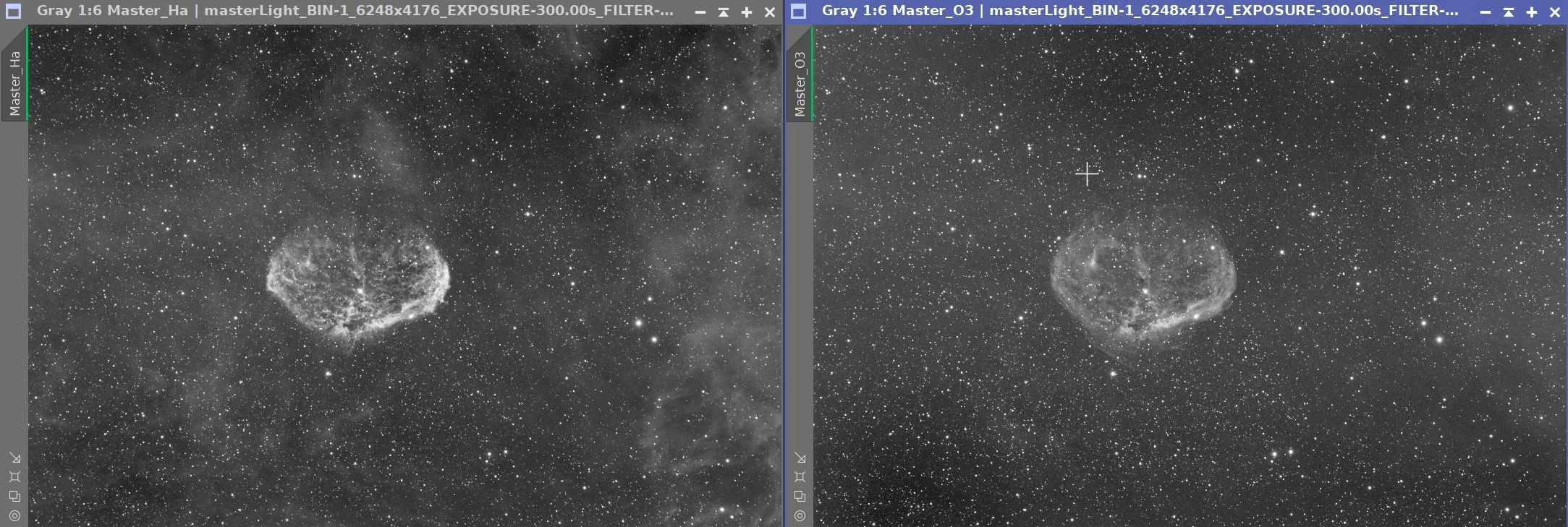
Initial Master Ha and O2 linear images!

Initial Master Red, Green, and Blue linear images!
5. Crop all of the images
A common crop level was selected, and DynamicCrop was used to trim all of the master frames.
The edges were remarkably clean. Only a little had to be removed from the right edge.
6. Dynamic Background Extraction
DBE was run for each image using the subtraction method. Below are the Sampling plans, the before image, the after image, and the removed background images.
DBE: Ha Sampling (Click to enlarge)
Ha image Before DBE (click to enlarge)
Ha image After DBE (click to enlarge)
Ha background removed (click to enlarge)
DBE: O3 Image Sampling (Click to enlarge)
O3 Image Before DBE (click to enlarge)
O3 Image After DBE (click to enlarge)
O3 background removed (click to enlarge)
DBE: Red Sampling (Click to enlarge)
DBE: Green Sampling (Click to enlarge)
DBE: Blue Sampling (Click to enlarge)
Red image Before DBE (click to enlarge)
Green image Before DBE (click to enlarge)
Blue image Before DBE (click to enlarge)
Red Image After DBE (click to enlarge)
Green Image After DBE (click to enlarge)
Blue Image After DBE (click to enlarge)
Red background removed (click to enlarge)
Green background removed (click to enlarge)
Blue background removed (click to enlarge)
7. Rotate all Images 180 degrees
This gets to the more traditional presentation of this target.
8. Apply light Noise Reduction to the Ha and O3 Linear Master Images
Apply Noise XTerminator with a value of 0.5 and the linear mode box checked.


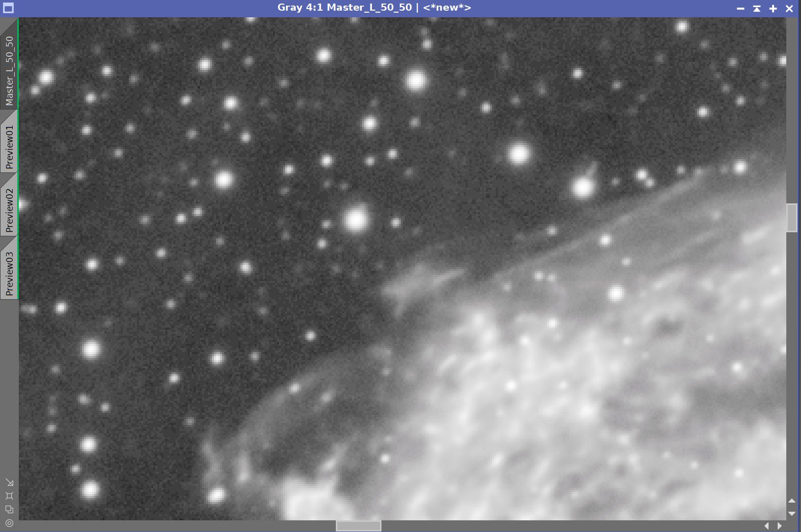
Master Linear Ha and O3 Images - Before and After Noise XTerminator 0.5 Linear
9. Create and Process the Synthetic Lum image
We only have two main data channels - Ha and O3 - so we can’t use ImageIntegration as it needs a minimum of 3.
So, the strategy is to add images together in a weighted fashion using PixelMath:
50% Ha + 50% O3
25% Ha + 75% O3
75% Ha + 25% O3
75% Ha + 25% O3 (click to enlarge)
50% Ha + 50% O3 (click to enlarge)
25% Ha + 75% O3 (click to enlarge)
With the 75%/25% Ha/O3 blend, you see the spikes at the top of the nebula but have completely lost the O3 shell.
With the 25%/75% Ha/O3 blend, you can see the O3 shell pretty well, but the Ha spikes are fading out.
The 50%/50% seems to be the best way to go.
10. Process the Linear Master L Image
Prep for Deconvolution
Run Psfmage and create the PSF file

The PFSImage Panel with settings used

The final PSF image
Run Starmask to create the initial LDSI image (see panel snap for parameters)

The StarMask panel set up to create the LDSI map.

The HT tool was used in this config to boost the LDSI image
Compare the mask to the original image - the stars are too small.
Apply HT Boost ( see panel snap for parameters) 2 or more times until star sizes match.

The Final LDSI image
Select Preview regions on the image for Decon exploration

These preview regions were selected to iteratively test the decon panel parameters for optimized results.
Iteratively run decon on previews until parameters are finalized (see panels snap for final values)

The final Deconvolution Parameters are shown

Master L - Before and After Deconvolution
11. Create the Master_RGB Image and Process
Create the RGB color image by using the ChannelCombination tool and the R, G, B Master Linear Images

Master R, G, and B images ready for combination

Master RGB image - initial
Run PCC on the RGB Image

Master RGB Image - After PCC

PCC Regression lines
Run DBE on the color image
Master RGB DBE Sampling plan (click to enlarge)
Master RGB - Before DBE (click to enlarge)
Master RGB After DBE (click to enlarge)
Master RGB Background Pattern (click to enlarge)
Run Noise XTerminator with a value of 0.5 and the Linear box checked.
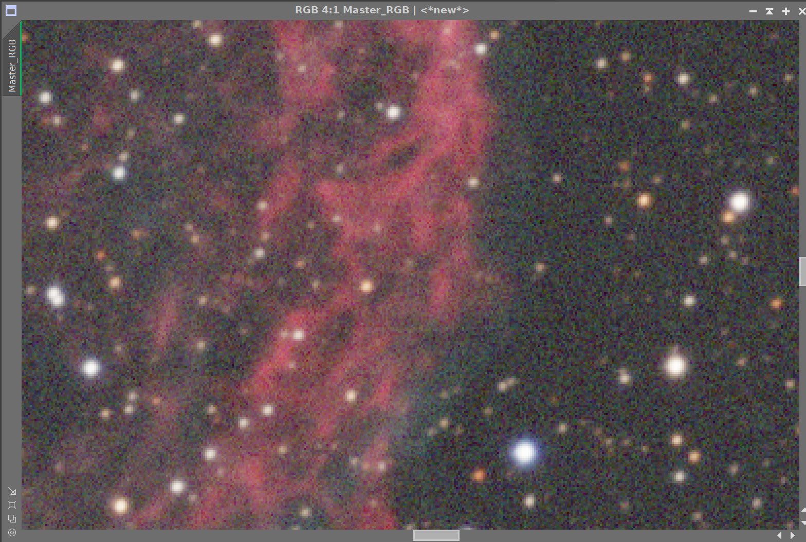

Master RGB - Before and After Noise XTerminator 0.5
12. Convert All Images to Nonlinear
Nonlinear RGB
Select a preview sample of the background sky
Run MaskedStetch with default values and the preview reference above.
Apply CT to adjust the color and tone scale
Nonlinear RGB after Masked Stretch (click to enlarge)
Nonlinear RGB after CT to adjust color and tone scale (click to enlarge)
Create a copy of the image using Blanhan’s First PM script
Run Starnet2 on it and create the Starless Image.
Apply Blanshan Method 2 with a value of 0.35
Before Star Reduction (click to enlarge)
After Star Reduction (Click to Enlarge)
Create L, Ha, O3, and color HOO nonlinear Files
For L, Ha, and O3 Master Images
Make a copy and label with Nonlinear
Create a custom STF to make the image look good
Use the STF-> HT method to go nonlinear.
Apply CT to tweak
Nonlinear L image after HT and CT (click to enlarge)
Nonlinear Ha after HT and CT (click to enlarge)
Nonlinear O3 after HT and CT (click to enlarge)
Create the first HOO color image
Linfit - O3 as reference - applied to Ha
Use ChannelCombination to create the HOO Image
Use CT to adjust the red curve
The initial Nonlin Ha image (click to enlarge)
Ha after Linfit using O3 as a reference (click to enlarge)

The O3 image that was used as the linfit reference (click to enlarge)
Initial HOO image (click to enlarge)
The HOO image after using CT to boost the red curve a bit (click to enlarge)
13. Take L image starless and Process
Create a starless version of the image by running Starnet2 on it.

Starless version of the Nonlin L image
Create a range mask to isolate the nebula
Use the RangeSlection process to make the initial Mask
Remove mask elements outside of nebula with the DynamicPaintBrush
Edit the nebula area of the mask to include O3 lobe at the top of the image
Smooth the mask out by running convolution with a sigma of 10, 5 times
Initial Range Mask (click to enlarge)
Edit the mask to expand the top to include the O3 lobe (click to enlarge)
Range Mask after elements outside of nebula are removed with DynamicPaintBrush (click to enlarge)
FInal Range Mask after blurring (clikc to enlarge)
Enhance detail in the nebula
Apply the final Nebula range mask
Run LHE with radius=64, contrast limit = 2.0, Amount = 0.3, 8-bit histogram
Run LHE with radius=370, contrast limit = 2.0, Amount = 0.3, 12-bit histograms
Sharpen with MLT (see screen snap below)
Starless L image after first LHE application for smaller scale structures (click to enlarge)
Starless L after the second LHE application for larger-scale structures..(click to enlarge)
Starless L after Sharpening (click to enlarge)

Here is the sharpening parameters used
14. Take HOO image Starless and Process
Create a Starless Version of the color HOO image
Do this by running starnet2
Use LRGBCombination tool to fold the Starless L image into the Starless HOO image
Run CT and adjust Tone and Color
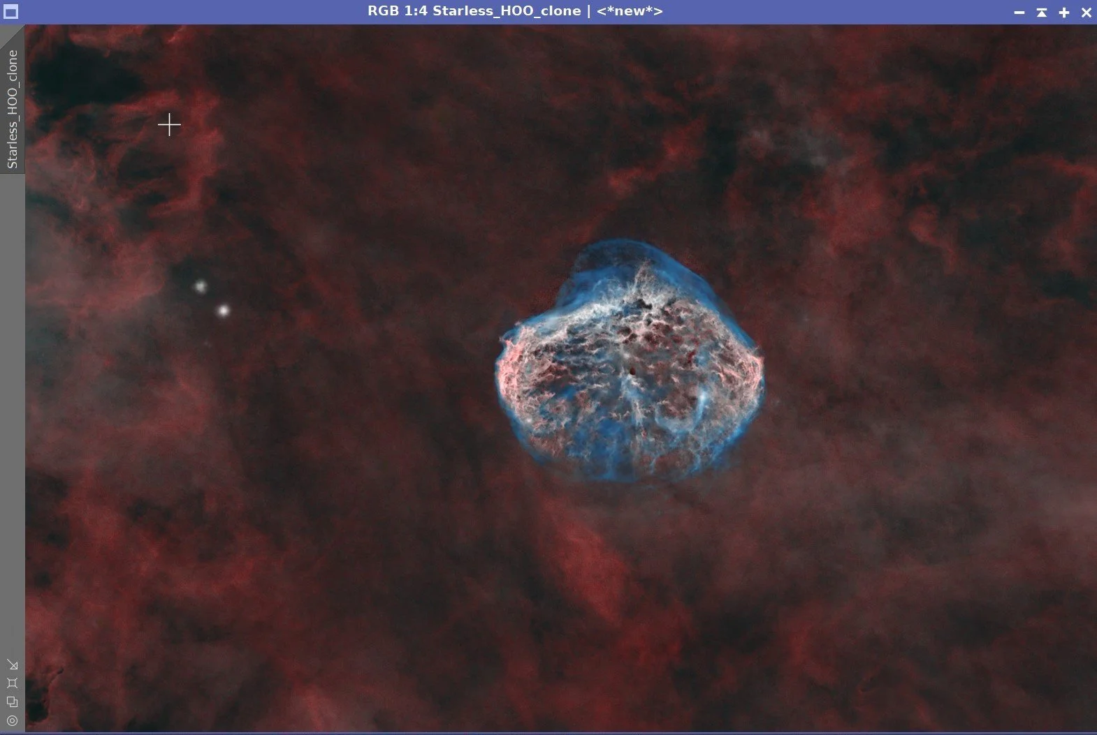
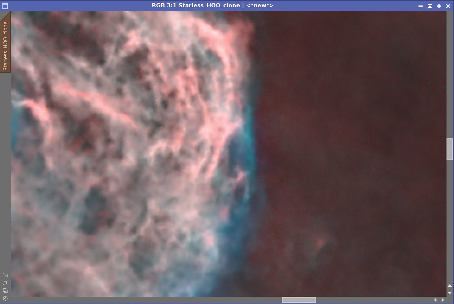
HOO Starless image - the starting point. (click to enlarge)
Starless L image folded in with LRGBCombination (click to enlarge)
HOO Starless after CT Adjustment (click to enlarge)
Create Masks needed for processing
Cyan mask
Run the Blanshan Cyanmask PM script
Boost with CT
Edit out everything but the nebula with the DynamicPaintBrush
Run the Blanshan blur script
Starting Cyan Mask (click to enlarge)
Cyan Mask boosted with CT (click to enlarge)
Final Mask after editing with DynamicPaintBrush and blur (click to enlarge)
Red mask
Run the Blanshan RedMask PM script
CT boost
Run Blanshan blur
Initial Red Mask (click to enlarge)
Red Mask Boosted with CT (click to enlarge)
Red Mask Blurred (click to enlarge)
Process using the Cyan mask
Run CT with Cyan mask and adjust the color and tone scale of the O3 regions
Run Noise XT on just the O3 regions - be aggressive with a 0.9 parameter
Process using the Red Mask
Run CT with Red Mask
Apply the Cyan Mask and Adjust O3 regions with CT (click to enlarge)
Apply the Red Mask and adjust with CT (click to enlarge)
15. Create RGB Stars Image
Run Starnet2 on the nonlinear RGB Stars image - click create star map
RGB Stars image after Starnet2 application (click to enlarge)
16. Recombine Stars and Starless Images
I tried using the StarBlend script, but it failed due to all of the red background nebula
So I went old school and just added the RGB Stars and the HOO Starless image together using PixelMath
Starless and Stars images added back together (click to enlarge)
17. Image Assessment
At this point, I studied the image. I was not happy on several fronts:
The brighter stars are bloated - even though they are quite small in the Stars-only image. This is because there is residual star bloat from the starless image coming through. I think this can be fixed by using clone-stamp on the starless image.
There is not enough contrast on the whole image
I still see some noise in the red background and especially in the O3 areas
So, I will go back to a place before the stars were added and do some extra work.
18. Stepping Back a Bit to Address Some Issues
Apply the Cyan Mask and run a light convolution run, with sigma=4 - to smooth out the O3 areas.
A slight convolution run done on O3 regions.
Run Noise XTerminator on the whole image with a value of 0.65

Before and After Noise XTerminator 0.65 run.
Apply the Range Mask and adjust color and tone with CT
Invert the Range Mask and adjust color and tone with CT
Adjust nebula with CT for color and tone scale (click to enlarge)
CT used to adjust the inverted Red Mask - tweaking the background (click to enlarge)
Remove the residual Stars from the HOO Starless image with the CloneStamp tool.
Add stars back in with PixelMath with a simple image addition.
Bright Star residuals removed with CloneStamp (click to enlarge)
Stars are now added back in. No more bloated stars, and the image is quite improved!
19. Export to Photoshop
Save images as Tiff 16-bit unsigned and move to Photoshop
There was not a lot to adjust here
I tweaked things with the camera filter clarity and curves
Based upon feedback, I also
Brightened and enhanced the brightest stars - I think I went too far before!
I cropped it tighter and rotated the image a bit.
Export Clear, Watermarked, and Web-sized jpegs.
The final image!
Adding the next generation ZWO ASI2600MM-Pro camera and ZWO EFW 7x36 II EFW to the platform…